Scrambling a Cat: A Tour of Modular Image Encryption

Explore confusion, diffusion, entropy, and avalanche effects in image encryption.

I built a small image-encryption playground where you upload a picture, pick some building blocks, and watch the image dissolve into noise and come back again. My test image, for reasons that will become clear, is a blurry cat glaring at an empty food bowl. By the end of this post you will understand exactly why that cat turns into static, why the static turns back into a cat, and which of the techniques involved is actually pulling its weight.

Before we start, an important caveat: this is an educational framework for studying confusion and diffusion. It is not a production-ready cryptographic system, and it has not undergone formal cryptanalysis. The goal is comparison, not deployment.

Why I built this

I originally built this project because most image-encryption papers compare algorithms only through tables of metrics. I wanted something more intuitive: a playground where I could swap components, watch every intermediate step, and see exactly which module was responsible for which security property.

Why images need their own treatment

If you encrypt a text file with a weak scheme, the damage is invisible to the naked eye. With images it is the opposite: a weak scheme leaves the picture recognizable. Neighboring pixels in a natural photo are highly correlated (the patch of fur next to a fur pixel is almost certainly more fur), so the data has enormous local structure. A good image cipher has to destroy two things at once:

1. The structure: where things are, the edges, the shapes.

2. The statistics: the fact that some pixel values are far more common than others.

Claude Shannon described two properties that strong ciphers need: confusion and diffusion. In image encryption, I find it helpful to think of them visually:

• Confusion: scramble where pixels are.

• Diffusion: scramble what pixel values are.

The whole pipeline is just these two stages, applied in turn, repeated for a few rounds.

The pipeline

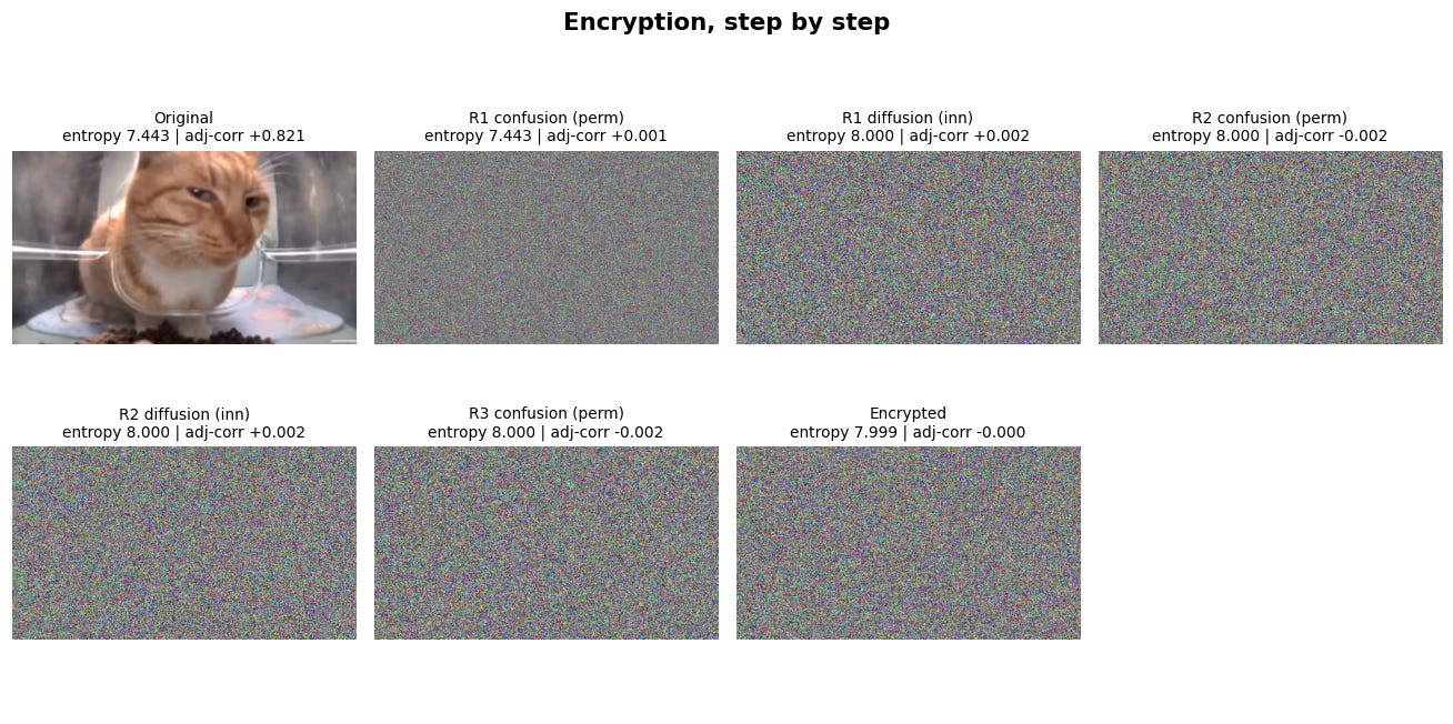
The image is flattened into a single list of bytes. Then, for each round, it runs one confusion stage followed by one diffusion stage. After R rounds you have the ciphertext. Decryption runs the rounds backward, undoing diffusion and then confusion at each step, and you get the exact original image back. Lossless, every time, for grayscale, color, and odd sizes.

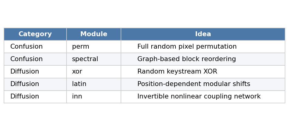
The interesting design choice is that confusion and diffusion are each a pluggable slot. I wrote two confusion modules and three diffusion modules, and any pairing works. That is what makes it a comparison rather than a single algorithm. Here are the five building blocks at a glance before we dig into each one:

A note on keys before the modules: every stage derives its own subkey. A label like inn3.2 (meaning the diffusion in round 3, coupling layer 2) is hashed together with your secret key using SHA-256, and the result seeds a dedicated random generator for that stage. So one master key fans out into dozens of independent stage keys, and nothing is reused between positions or rounds.

The confusion modules: scrambling positions

Confusion only moves pixels around. It never changes the actual values, so the histogram and the global entropy stay exactly the same. What collapses is the spatial pattern and the correlation between neighboring pixels.

perm: the honest shuffle

The baseline. Seed a random generator from the key, generate a full random permutation of every pixel index, and reorder the image by it. To decrypt, apply the inverse permutation. It is the most thorough scrambler you can ask for, because it treats every pixel independently and can send any pixel anywhere. Its only shortcoming is conceptual: it knows nothing about the image being an image.

spectral: scrambling with a sense of geometry

This is the more interesting confusion idea. Instead of shuffling individual pixels, it shuffles blocks. The image is cut into an 8 by 8 grid of tiles. Then the key builds a small graph over those 64 tiles (a symmetric matrix of random edge weights that depends only on the key, never on the image content). From that graph it computes the Fiedler vector, the eigenvector tied to the second-smallest eigenvalue of the graph Laplacian. The Fiedler vector is the classic signal used in spectral clustering to lay out a graph along a line, and here it gives a key-dependent ordering of the blocks. The tiles get reshuffled into that order, and decryption restores the original order. If the image is too small to fill the grid, it quietly falls back to perm.

The diffusion modules: changing values

Diffusion is where the histogram gets flattened and entropy climbs toward its ideal of 8 bits per pixel. It is also where resistance to differential attacks lives, which I will measure below.

xor: the textbook keystream

Generate a key-seeded stream of random bytes as long as the image and XOR it into the pixels. XOR is its own inverse, so decryption is the identical operation. It flattens the histogram nicely, but it is linear and each byte is mixed in isolation, so by itself it gives no avalanche: changing one input pixel changes exactly one output pixel.

latin: balanced, analyzable, and deliberately weak

This one adds a position-dependent shift to each pixel: position i gets (a * i + b) mod 256, where a is forced to be odd so the operation is reversible modulo 256, and b is a keyed offset. The result is provably balanced, meaning each output value is equally likely across positions, which makes it clean to reason about. But it is still a linear function of position, so it is the intentionally weak diffusion arm. Having a weak baseline matters: the comparison is only meaningful if something loses.

inn: the strong contender

The centerpiece is an integer coupling network, borrowing the additive-coupling trick from RealNVP (a normalizing-flow architecture) and adapting it to be exactly invertible over bytes. Here is the idea:

1. Split the vector into two halves, a and b.

2. Compute a shift t from a using a keyed, causal, nonlinear mixer. Each t_i depends on the key and on every earlier value of a through a running accumulator, then passes through a key-seeded 8-bit substitution box.

3. Update the other half: b = (b + t) mod 256.

4. Swap the two halves and repeat for several layers.

The magic of coupling networks is that step 2 reads only the half that is not being changed. So at decryption time you can recompute the identical t and subtract it, and the whole thing inverts perfectly, no matter how nonlinear the mixer is. The causal accumulator is what creates real avalanche: flip one early pixel and every later output shifts. That property is exactly what the differential metrics reward.

How do you know it worked?

Four numbers, computed on the cat and its ciphertext.

• Entropy measures how uniform the pixel histogram is. The ideal is 8.0 bits per pixel, meaning every byte value is equally likely and there is no statistical handle to grab. The cat starts at about 7.44.

• Adjacent-pixel correlation measures how much a pixel predicts its neighbor. Natural images are strongly correlated; the cat sits around +0.82. A good cipher drives this to roughly zero.

• NPCR (Number of Pixel Change Rate): flip one pixel of the input, encrypt both versions, and count what fraction of output pixels differ. The ideal is about 99.6 percent.

• UACI (Unified Average Changing Intensity): same setup, but it measures the average intensity of the change, not just whether a change happened. The ideal is about 33.4 percent.

NPCR and UACI together are the differential-attack story: they say that a tiny nudge to the input produces a totally different output, so an attacker cannot learn anything by feeding in near-identical images.

Results

Running perm confusion with inn diffusion for 3 rounds:

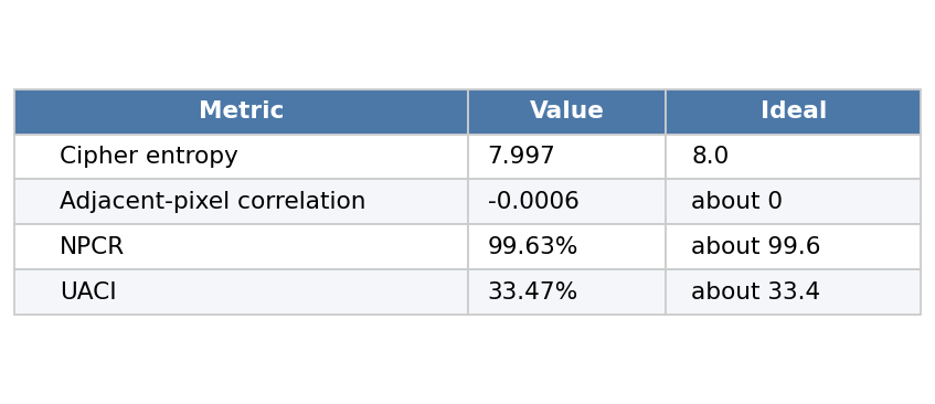
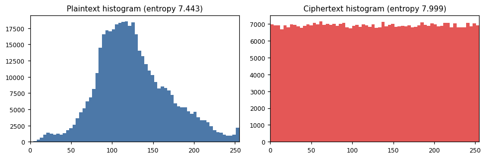
The cipher histogram goes flat, the correlation collapses from +0.82 to essentially nothing, and the differential numbers land right on their ideals. The avalanche from the inn coupling network is what carries those last two. If you swap inn for the linear latin module, the differential numbers degrade noticeably, which is the comparison the project was built to show.

The moment that surprised me

The app shows every intermediate stage, and the decryption gallery taught me something I did not expect. None of the steps look even slightly like the cat until the very last one. It is full rainbow static, then full static, then suddenly a cat.

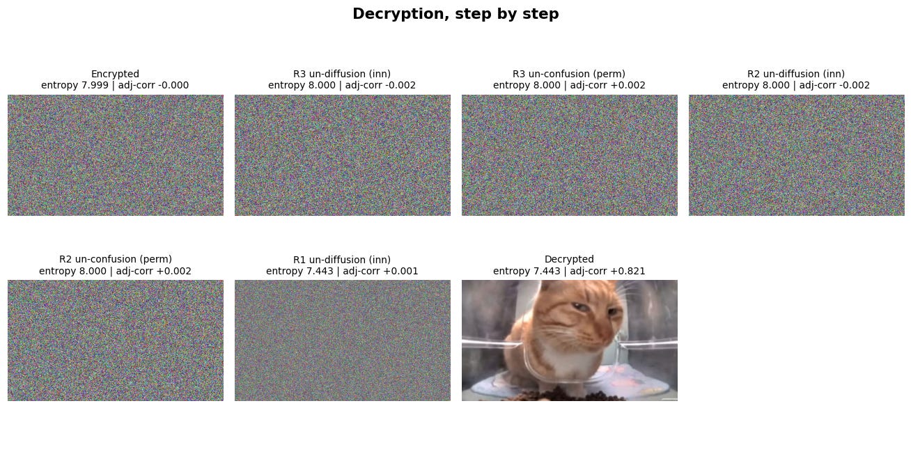
That is not a bug, it is the goal. The image is only recognizable when the values and the positions are simultaneously correct. Decryption fixes those separately: un-diffusion restores the values, un-confusion restores the positions, and because confusion ran in every round, the pixels stay scrambled until the final un-confusion. There is one beautiful tell, though. The second-to-last step looks grayer and smoother than the others. At that moment the pixels are the cat’s exact values, just shuffled into the wrong places, so the tile carries the cat’s muted color palette and its entropy drops from 8.0 back to 7.44. That step is the cat, spatially scrambled. The final step just puts every pixel back where it belongs.

If you could see the cat slowly fading in across the steps, that would actually be bad news: it would mean structure was leaking out early. The fact that it snaps from noise to image in a single step is the visible signature of strong confusion and diffusion working together.

What I would do next

A few honest limitations and directions:

• These are learning primitives. They are useful for studying confusion and diffusion behavior, not for protecting anything that matters.

• The latin arm is linear on purpose, and a real attacker would exploit that. It earns its place as the baseline that the comparison beats.

• Natural next steps: a perceptual or latent-space stage (encrypting in the latent space of an autoencoder), and a robustness battery (chosen-plaintext, cropping, and noise tolerance) that reviewers always ask for.

Try it

The code, the metrics harness, and the Streamlit app are all on GitHub: Modular-Image-Encryption.

The cat is just the default image. Any photo works. Pick a confusion module, pick a diffusion module, choose a few rounds, and watch how quickly recognizable structure disappears. Then reverse the process and see how much work it takes to turn pure noise back into a cat.